
Frequently, investigators need to know more than the end result, the final yield of dry matter. Events along the way may have had a marked influence on the final outcome. One approach to the analysis of yield-influencing factors and plant development as net photosynthate accumulation is naturally integrated over time has come to be known as growth analysis.
The basic concept and physiological implications in growth analysis are relatively simple and have been explained in the early classic approaches by V. H. Blackmail (1919), Briggs et al. (1920), and Fisher (1920).
Growth analysis came to be used extensively in the British Commonwealth countries, including the classic work of Watson (1947, 1952). In recent years growth analysis has been used by plant physiologists and agronomists in the United States. Two extensive treatments of the subject have been published.
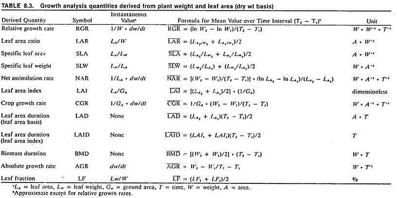
Only two measurements, made at frequent intervals, are required for growth analysis- leaf area and dry weight. Other quantities in the analysis are derived by calculation (Table 8.3). The commonest approach, classic growth analysis, involves measurements made at fairly long intervals (1-2 wk) on a relatively large number of plants.
The second approach involves measurements at more frequent intervals (2-3 days) on a smaller number of plants. Both approaches provide mean values of the quantitative changes that occur over any particular time interval. The second approach, using more frequent harvests, has been suggested to make better use of the materials and time of the researcher.
Dry weight is determined by standard procedures. Leaf area (one side only) can be determined a number of ways. Currently the commonest is by a photoelectric device that reads leaf area directly as individual leaves are fed into it. Another common method is using linear regression analysis: area = a + b (I × w), where b = slope, l = leaf length, and w = leaf width.
From regression analysis on 60 leaflets, the author obtained the equation for leaf area determination of bush bean- a = .624 + .583 (l × w). Equations for most crop plants have been published.
Other methods of leaf area determination include tracing fresh leaves on grid, blueprint, or photocopy paper to determine area-weight ratio. The leaf weight experimentally determined can then be converted to leaf area by calculation. Other quantities for the growth analysis can be calculated (Table 8.3). Growth analysis can be made of individual plants or of plant communities.
Analysis of individual plant growth, generally made at the early stages, includes the following:
(1) Relative and absolute growth rates
(2) Unit leaf rate or net assimilation rate
(3) Leaf area ratio
(4) Specific leaf area
(5) Specific leaf weight and allometry in growth (e.g., S-R ratio) (Table 8.3).
1. Relative Growth Rate:
Relative growth rate (RGR) expresses the dry weight increase in a time interval in relation to the initial weight. In practical situations, the mean relative growth rate (R̅G̅R̅) is calculated from measurements taken at times and t2. The equation for calculating the RGR is derived from the compound interest equation, W = W0ert, where W is the weight at any given time, W0 is the initial weight, e is the natural logarithm base (2.71828), r is the relative growth rate, and t is the length of the time period. The R̅G̅R̅ does not imply a constant growth rate during a particular t1, to t2 time frame; it can vary from instantaneous values of RGR. RGR is the slope of the line when log, W is plotted against t.
The example in Table 8.4 shows that plants A and B had the same RGR, although B gained 10 g and A gained 5 g. This is because B was twice as large at the start. The RGR of crop plants generally begins slowly just after germination, peaks rapidly soon afterward, and then falls off. Species vary in RGR.
For example, during a 5 wk period from germination Grime and Hunt (1975) observed a wide distribution of RGRs among woody and herbaceous species under favorable conditions. The maximum instantaneous R̅G̅R̅s ranged from a low of 0.22 g. g-1.wk-1 for Sitka spruce to a high of 2.70 g. g-1.wk-1 for Poa annus (annual bluegrass).
2. Leaf Area Ratio:
Leaf area ratio (LAR) expresses the ratio between the area of leaf lamina or photosynthesizing tissue and the total respiring plant tissues or total plant biomass (Table 8.3). The LAR reflects the leafiness of a plant, but mean values (L̅A̅R̅) were not precise.
Plants like sunflower and beet had a high LAR, compared with plants like pine, and also had a 10-fold greater RGR. Such differences suggest, all other factors being equal, a strong competitive position for sunflower in the juvenile stages.
3. Net Assimilation Rate:
Net assimilation rate (NAR), or unit leaf rate, is the net gain of assimilate, mostly photosynthetic, per unit of leaf area and time. It also includes gain in minerals, but this is not a large fraction since minerals constitute only 5% or less of the total weight.
The equation to calculate mean values (NAR) (Table 8.3) assumes that the relationship between plant weight and leaf area is linear; this assumption may hold for early phases of ontogeny but not for latter phases, as growth rate of leaf area may exceed that of dry matter or vice versa.
NAR is not constant with time but shows an ontogenetic downward drift with plant age. The age drift was accelerated by an unfavorable environment and dry matter- gain per unit leaf surface decreases as new leaves are added due to mutual shading. Increased competition for nutrients and other factors are probably also important as age and size increase.
Agronomists generally analyze plant community growth, since it represents the accumulation of economic yield.
Quantities used in growth analysis of plant communities include:
1. Leaf Area Index
2. Crop Growth Rate
3. Crop growth rate of total biomass (usually the above-ground parts) and of the economic biomass (e.g., seeds, tubers).
4. Net assimilation rate
The partitioning coefficient or index can be calculated as a ratio between the economic biomass and the total biomass. A complete growth analysis evaluates both the individual plant and the plant community. The formulas, symbols, and other information for calculating the quantities derived in growth analysis are given in Table 8.3.
1. Leaf Area Index:
Crop production is the practical means of trapping solar energy and converting it into food and other usable materials. Crop production strategies are usually designed to maximize light interception by achieving complete ground cover through manipulating plant density and spatial arrangement and promoting rapid leaf expansion. Bare ground does not trap and convert light energy.
Leaf area index (LAI) expresses the ratio of leaf surface (one side only) to the ground area occupied by the crop. Mean values (L̅ I̅A̅) are calculated in Table 8.3. A LAI of 1, which is one unit of leaf surface area per unit of land surface, theoretically could intercept all incident light; but it seldom does, due to leaf shape, thinness (light is transmitted), inclination, and vertical distribution variations. A LAI of 3-5 is usually necessary for maximum dry matter production of most cultivated crops.
Forage crops, such as grasses, with erectophile (upright) leaf orientation may require a LAI of 8-10 under favorable conditions to maximize light interception. A higher LAI is also required where total biomass, not economic yield, is the objective (e.g., forage crops). In this case assimilate in excess of growth and maintenance respiration in amounts sufficient to produce seeds or tubers are not required or desired.
The LAI and its seasonal distribution vary considerably with species. Values required for maximum production increase with the level of solar radiation.
2. Crop Growth Rate:
Crop growth rate, the gain in weight of a community of plants on a unit of land in a unit of time, is used extensively in growth analysis of field crops. See Table 8.3 for a calculation of the mean value (C̅G̅R̅). A (C̅G̅R̅) of 20 g. m-2 .day-1 (200 kg. ha-1. day-1) is considered respectable for most crops, particularly C3 types. A CGR of 30 g. m-2 .day-1 (300 kg. ha-1. day-1; for grain, 6 bu. a-1 . day-1) is obtainable from C4 types, such as maize.
The CGR of economic yield, such as grain or tubers, is of equal or greater interest. When the total and economic dry weights are plotted against time, the slope of the regression line of the linear phase (slope = CGR) is usually similar for high-yielding cultivars. The ratio of CGRecon to CGRtotal produces a useful quantity, referred to as the partitioning coefficient or index.
The partitioning coefficient of a crop expresses efficiency in conversion of assimilate to economic yield. Modern cultivars of peanut partitioned at about 75%, some of the older cultivars at only 40 to 50%. The nut yields from new peanut cultivars, such as ‘Florunner’ are about twice those from ‘Dixie Runner’ and other older cultivars with low partitioning coefficients.
3. Leaf Area Duration:
Leaf area duration (LAD) expresses the magnitude and persistence of leaf area or leafiness during the period of crop growth. It reflects the extent or seasonal integral of light interception and in wheat has been shown to correlate highly with yield.
Mean leaf area duration (L̅A̅D̅) is calculated from the leaf area from individual plants (Table 8.3). In field crops the primary interest is the relationship of leaf area to land surface, or LAI, and L̅A̅D̅ can also be calculated on this basis (Table 8.3).
If LAI is plotted against time, it produces a function that indicates the crop’s assimilatory capacity during the period in question. Using four crops — barley, potato, wheat, and sugar beet —Watson (1947) found that the N̅A̅R̅s during periods of rapid growth were quite similar but that the L̅A̅D̅s for the four crops differed significantly.
4. Biomass Duration:
Biomass duration (BMD) (Table 8.3) is analogous to LAD. If the area under the time curve for biomass production is calculated as explained for LAD, the value for biomass persistence with time is obtained. This quantity may be less useful when used alone than in the calculation of maintenance respiration losses over time, a function of live weight and temperature.
Those and other derived quantities can assist in better understanding crop responses. They can be used to construct models of plant responses to measurable parameters. McCollum (1978) applied growth analysis to the data obtained from potato grown at different soil phosphorus (P) levels.
Growth curves for plants with adequate P were sigmoid and exhibited four post emergence ontogenetic phases:
(1) Pretuber vegetative (emergence to 28 days).
(2) Tuber initiation, bulking, and rapid leaf growth (28-50 days).
(3) Continued tuber growth and leaf loss.
(4) Death of haulms (50-80 days).
Plants with low P never entered phase 3. Low-P plants developed only 50% of the LAI, had a reduced NAR in the early growth phases and had a reduced LAD, compared with high-P plants.
No comments yet.